Dark Worlds Challenge
Posted on February 08, 2018
Observing Dark Worlds was a Kaggle competition from 2012 the goal of which was to develop algorithm for predicting location of dark matter. To detect dark matter aggregations in deep space, astrophysicists inspect the change in visual appearance of background galaxies. Dark matter distorts spacetime and causes light to bend when passing through forming the so-called halos. As a result, background galaxies appear more elongated than they actually are, an effect known as gravitational lensing. The observed ellipticity of galaxies correlates with the position of dark matter halos and makes it possible to estimate these positions.
See A Beginners Guide to Dark Matter by David Harvey for more details on the data and the problem of identifying dark matter halos.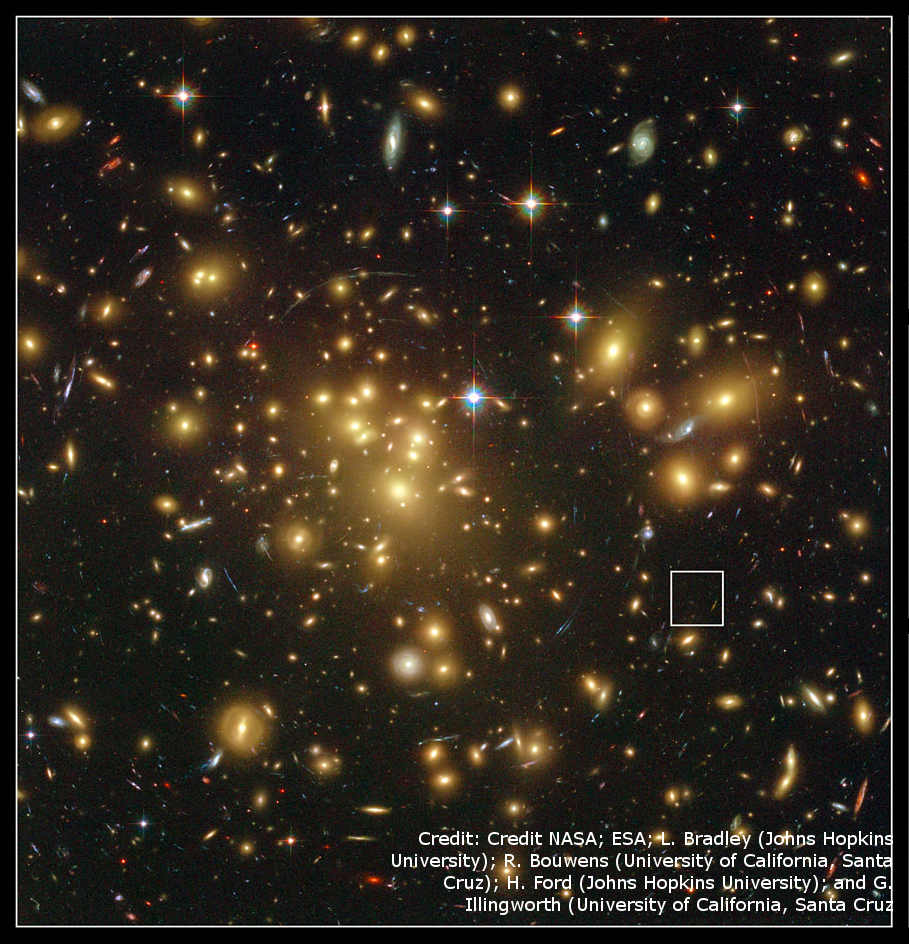
The organizers of the competition provide a training database with 300 sky maps, Training_Sky1 to Training_Sky300. Each map contains coordinates of galaxies in the sky map, variables x and y, along with their observed ellipticity, variables e1 and e2. There are between 300 and 700 galaxies in each training map. The file Training_halos.csv provides the true halo locations in each map. There may be up to 3 halos in a map. A separate set of 120 test maps, Test_Sky1 to Test_Sky120, is used for evaluation of prediction performance.
In this post I discuss a Bayesian approach to the problem but I don't provide a complete solution. My goal is to show how one can leverage the label information in the training data to fine-tune the hyperparameters in a posterior model which can then be applied to test data. The approach can be generalized to other supervised learning problems.
Likelihood model
I follow the guidelines suggested here to formulate the likelihood function for the observed galaxy ellipticity.The effect of a dark-matter halo positioned at \((x', y')\) on a galaxy located at \((x, y)\) is given by a pair of tangential ellipticity coefficients \((te_1, te_2)\) according to
\begin{align}
\begin{split}
te_1 = -\cos(\phi) \\
te_2 = -\sin(\phi) \\
\phi = 2\arctan(\frac{y-y'}{x-x'})
\end{split}
\end{align}
From the tangential ellipticity we obtain the observed ellipticity \((e_1, e_2)\) which is proportional to the mass of the halo \(m\) and inversely proportional to the Euclidean distance \(\rho\) between the galaxy and the halo
\begin{align}
\begin{split}
e_1 = -m\cos(\phi)/\rho \\
e_2 = -m\sin(\phi)/\rho \\
\end{split}
\end{align}
The halo mass m is unknown and has to be included as a model parameter. I decide to model it in the log-scale by a parameter lm, thus \(m = \exp(lm)\). That will give me more flexibility in specifying a prior for the mass. Let \(r = 1/\rho\) be the inverse distance between the galaxy and the halo. As noticed by some of the winners in the competition, Tim Salimans and others, it is beneficial to put some lower limit for the distance \(\rho\). This prevents \(r\) from blowing up when the distance gets close to 0 and makes the model more stable. Instead of using the trial and error approach to find an optimal limit, I include it in the model and let it be estimated using the training data. Let the hyperparameter \(rmax\) be the upper limit for \(r\). The ellipticity equations then become
\begin{align}
\begin{split}
e_1 = -\exp(lm)\cos(\phi)\min(rmax, r) \\
e_2 = -\exp(lm)\sin(\phi)\min(rmax, r) \\
\end{split}
\end{align}
It is reasonable to assume that the observed ellipticity include some measurement error modeled by a Gaussian noise with variance given by a parameter \(sig2\). I can then write the likelihood of my model
\begin{align}
\begin{split}
e_1 \sim \mathcal{N}(-\exp(lm)\cos(\phi)\min(rmax, r), sig2) \\
e_2 \sim \mathcal{N}(-\exp(lm)\sin(\phi)\min(rmax, r), sig2)
\end{split}
\end{align}
The errors for \(e_1\) and \(e_2\) are assumed uncorrelated.
bayesmh (e1=(exp({lm})*{cos2t:}*{r:})) (e2=(exp({lm})*{sin2t:}*{r:})),
	likelihood(mvnormal({sig2}))
	define(dx: x-{halox}) define(dy: y-{haloy})
	define(cos2t: ({dy:}^2-{dx:}^2)/({dy:}^2+{dx:}^2))
	define(sin2t:-2*{dx:}*{dy:}/({dy:}^2+{dx:}^2))
	define(r: min({rmax}, 1/sqrt({dy:}^2+{dx:}^2)))
        ...
There are 5 model parameters: {halox} and {haloy}, the coordinates of the unknown halo, {rmax}, {lm}, and {sig2}. I am using {dx:} and {dy:} as placeholders for the coordinate differences between the galaxies and the halo, {cos2t:} and {sin2t:} for the tangential ellipticity coefficients \(te_1\) and \(te_2\), and {r:} for the minimum of the inverse distance \(r\) and \(rmax\).
Supervised and unsupervised Bayesian models
My approach to Bayesian supervised learning goes through two Bayesian models. The first model utilizes the true halo coordinates available in the training data to elicit information about the parameters {rmax}, {lm} and {sig2}. In the second model, I use this information to build a unsupervised model where the halo coordinates are assumed unknown and will be estimated from the observed galaxy ellipticity. Of course, only the second model is applicable to test data.
In the supervised model, I assume that the true halo coordinates {halox} and {haloy} are normally distributed with means halox and haloy, the estimated coordinates available in the training data, and variance {sig2}:
  ...
  prior({halox}{haloy}, mvnormal(2, halox, haloy, {sig2}))
  ...
Note that the variance {sig2} is the same one used in the likelihood
function. This choice is based on the assumption that the halo and
ellipticity estimations are subject to the same observation error, which is not
unreasonable. Lets apply a vague inverse-gamma prior for the variance {sig2}:
igamma(0.1, 0.1).
Given the dimensions of each map, a local distance of 10 should be considered small. I therefore expect {rmax} to be less than 0.1 and I assign it a uniform(0.001, 0.1) prior. Finally, I assume that the halo's log-mass follows a normal prior with mean 1 and variance 10. These all seem to be innocuous assumptions. Here it is the complete model specification using the bayesmh command
bayesmh (e1=(exp({lm})*{cos2t:}*{r:})) (e2=(exp({lm})*{sin2t:}*{r:})),
	likelihood(mvnormal({sig2}))
	define(dx: x-{halox}) define(dy: y-{haloy})
	define(cos2t: ({dy:}^2-{dx:}^2)/({dy:}^2+{dx:}^2))
	define(sin2t:-2*{dx:}*{dy:}/({dy:}^2+{dx:}^2))
	define(r: min({rmax}, 1/sqrt({dy:}^2+{dx:}^2)))
	prior({rmax},  uniform(0.001, 1))
	prior({lm},    normal(1, 10))
	prior({halox}{haloy}, mvnormal(2,
                              `=mhalo1[1,2]',`=mhalo1[1,3]', {sig2}))
	prior({sig2}, igamma(0.1, 0.1))
In the second model, I assume that the unknown halo coordinates {halox} and {haloy} follow a completely uninformative prior: uniform(0, 4200), where (0, 4200) is the observed coordinate range in the sky maps.
Finding the halo in the first sky
Lets apply the supervised Bayesian model formulated above to the first training sky map. I first need to load the file containing the known halo coordinates
. import delimited data/Training_halos.csv
. summarize

    Variable |        Obs        Mean    Std. Dev.       Min        Max
-------------+---------------------------------------------------------
       skyid |          0
 numberhalos |        300           2    .8178608          1          3
       x_ref |        300    2148.174    1088.439      27.72     4169.9
       y_ref |        300     2207.16    1106.727        .62    4197.65
     halo_x1 |        300     2153.49    1189.761      10.24    4188.56
-------------+---------------------------------------------------------
     halo_y1 |        300    2220.473    1214.173        .62    4197.65
     halo_x2 |        300    1425.036    1397.369          0       4166
     halo_y2 |        300     1414.77    1419.384          0    4162.19
     halo_x3 |        300    678.4122     1211.98          0    4178.54
     halo_y3 |        300    651.0135    1190.116          0    4185.87
To simplify the case, I only consider maps with 1 halo, so I create a matrix
mhalo1 containing the indices and halo coordinates for the 1-halo sky maps
. set seed 12345
. gen skyid1 = _n*(numberhalos==1)
. mkmat skyid1 halo_x1 halo_y1 if skyid1>0, mat(mhalo1)
The halo coordinates in the first sky map, about 1087 and 1115, are given by the matrix entries mhalo1[1,2] and mhalo1[1,3]. I shall supply them to bayesmh using the local macros `=mhalo1[1,2]' and `=mhalo1[1,3]'.
Lets load the dataset of the first sky map which I know has 1 halo only
. import delimited data/sky/Training_Sky1.csvand simulate the first Bayesian model. In addition to the posterior options, I separate the parameters of interest, {rmax}, {lm}, and {sig2}, into individual blocks (expecting them to be fairly independent) and supply valid initial options. I furthermore request a MCMC sample of size 5000.
. set seed 1
. bayesmh (e1=(exp({lm})*{cos2t:}*{r:})) (e2=(exp({lm})*{sin2t:}*{r:})),  ///
	likelihood(mvnormal({sig2}))                                      ///
	define(dx: x-{halox}) define(dy: y-{haloy})                       ///
	define(cos2t: ({dy:}^2-{dx:}^2)/({dy:}^2+{dx:}^2))                ///
	define(sin2t:-2*{dx:}*{dy:}/({dy:}^2+{dx:}^2))                    ///
	define(r: min({rmax}, 1/sqrt({dy:}^2+{dx:}^2)))                   ///
	prior({rmax},  uniform(0.001, 1))                                 ///
	prior({lm},    normal(1, 10))                                     ///
	prior({halox}{haloy}, mvnormal(2,                                 ///
                              `=mhalo1[1,2]',`=mhalo1[1,3]', {sig2}))     ///
	prior({sig2}, igamma(0.1, 0.1))                                   ///
	block({lm}) block({rmax}) block({sig2})                           ///
	init({lm} 2 {rmax} 0.1 {sig2} 1)                                  ///
	mcmcs(5000) dots

Burn-in 2500 aaaaaaaaa1000aaaaaaaaa2000aaaaa done
Simulation 5000 .........1000.........2000.........3000.........4000.........50
> 00 done

Model summary
------------------------------------------------------------------------------
Likelihood:
  e1 e2 ~ mvnormal(2,exp({lm})*xb_cos2t*xb_r,exp({lm})*xb_sin2t*xb_r,{sig2})

Priors:
  {halox haloy} ~ mvnormal(2,1086.800048828125,1114.609985351563,{sig2})
         {rmax} ~ uniform(0.001,0.1)
         {sig2} ~ igamma(0.1,0.1)
           {lm} ~ normal(1,10)
------------------------------------------------------------------------------

Bayesian multivariate normal regression          MCMC iterations  =      7,500
Random-walk Metropolis-Hastings sampling         Burn-in          =      2,500
                                                 MCMC sample size =      5,000
                                                 Number of obs    =        348
                                                 Acceptance rate  =      .3927
                                                 Efficiency:  min =      .1143
                                                              avg =       .157
Log marginal likelihood =  85.417779                          max =      .1963

------------------------------------------------------------------------------
             |                                                Equal-tailed
             |      Mean   Std. Dev.     MCSE     Median  [95% Cred. Interval]
-------------+----------------------------------------------------------------
       halox |  1086.806   .2058405   .008609   1086.804   1086.383   1087.201
       haloy |  1114.601   .2135336   .008191   1114.597   1114.172   1115.018
        rmax |  .0530633   .0280319   .000905   .0537841   .0064036   .0978673
          lm |   3.84977   .2919037   .010786   3.894357   3.139424   4.279701
        sig2 |  .0450231   .0024271   .000077   .0449918   .0404852   .0501556
------------------------------------------------------------------------------
Unsurprisingly, the posterior mean estimates for {halox} and {haloy} match the true halo coordinates due to the prior we specified. My interest however is in the other 3 parameters. Posterior means and standard deviations of {rmax}, {lm}, and {sig2} provide us with important information about these parameters which is relevant for all other sky maps. For example, we see that the variance parameter {sig2} is about 0.045 and this is expected to be true for all other training and testing sky maps.
To formulate the second, unsupervised, Bayesian model, I use the posterior mean estimates for {rmax}, {lm}, and {sig2} from the first model to specify more informative priors. Lets save the posterior summaries of the parameters of interest in a matrix msum
. bayesstats summ {rmax} {lm} {sig2}
. mat msum = r(summary)
Now, the matrix entries msum[1,1] and msum[1,2] contain the posterior mean and standard deviations of {rmax}, which I use to specify an informative prior for {rmax}:
normal(`=msum[1,1]', `=msum[1,2]^2'))note that the standard deviation is squared. The entries msum[2,1] and msum[2,2] contain the posterior mean and standard deviations for {lm}, which I use to specify an informative prior for {lm}:
normal(`=msum[2,1]', `=msum[2,2]^2'))I also use the posterior mean of {sig2}, msum[3,1], to replace the variance parameter in the likelihood of the first model. As I mentioned above, the halo coordinates {halox} and {haloy} now have completely uninformative priors uniform(0, 4200).
What follows is the full specification of the second Bayesian model along with the simulation results.
. set seed 1
. bayesmh (e1=(exp({lm})*{cos2t:}*{r:})) (e2=(exp({lm})*{sin2t:}*{r:})), ///
	likelihood(mvnormal(`=msum[3,1]'))                               ///
	define(dx: x-{halox}) define(dy: y-{haloy})                      ///
	define(r: min({rmax}, 1/sqrt({dy:}^2+{dx:}^2)))                  ///
	define(cos2t: ({dy:}^2-{dx:}^2)/({dy:}^2+{dx:}^2))               ///
	define(sin2t:-2*{dx:}*{dy:}/({dy:}^2+{dx:}^2))                   ///
	prior({rmax}, normal(`=msum[1,1]', `=msum[1,2]^2'))              ///
	prior({lm},   normal(`=msum[2,1]', `=msum[2,2]^2'))              ///
	prior({halox}, uniform(0, 4200))                                 ///
	prior({haloy}, uniform(0, 4200))                                 ///
	init({lm} 1) block({lm}) mcmcs(5000) dots

Burn-in 2500 aaaaaaaaa1000aaaaaaaaa2000aaaaa done
Simulation 5000 .........1000.........2000.........3000.........4000.........50
> 00 done

Model summary
------------------------------------------------------------------------------
Likelihood:
  e1 e2 ~ mvnormal(2,expr6,expr7,.0450230840619126)

Priors:
  {halox haloy} ~ uniform(0,4200)
         {rmax} ~ normal(.0530632648891123,.0007857890494254)
           {lm} ~ normal(3.849770050209967,.0852077452213579)

Expressions:
  expr6 : exp({lm})*xb_cos2t*xb_r
  expr7 : exp({lm})*xb_sin2t*xb_r
------------------------------------------------------------------------------

Bayesian multivariate normal regression          MCMC iterations  =      7,500
Random-walk Metropolis-Hastings sampling         Burn-in          =      2,500
                                                 MCMC sample size =      5,000
                                                 Number of obs    =        348
                                                 Acceptance rate  =      .3793
                                                 Efficiency:  min =      .1038
                                                              avg =      .1466
Log marginal likelihood =  88.063805                          max =       .208

------------------------------------------------------------------------------
             |                                                Equal-tailed
             |      Mean   Std. Dev.     MCSE     Median  [95% Cred. Interval]
-------------+----------------------------------------------------------------
       halox |  1046.183   43.07794   1.84272   1049.074   944.8554   1123.163
       haloy |  1090.764   64.73769   2.84159   1092.794   952.1675   1202.468
        rmax |  .0559463   .0252325   .000783   .0552896    .010796   .1063793
          lm |  3.880156   .2010585   .006996   3.896191   3.461298   4.233885
------------------------------------------------------------------------------
The posterior mean estimates for the halo coordinates in the first sky map, about (1046, 1091), are very close to the true halo coordinates (1087, 1115). Of course, this is not so impressive given that we have used information from the first sky map to tune the priors for second model. Lets verify the validity of the model on independent data - the second training sky map.
. import delimited data/sky/Training_Sky2.csvThe second sky map also have only 1 halo and I know its true coordinates, (3478, 1907).
Lets run the same Bayesian model as above
. set seed 2
. bayesmh (e1=(exp({lm})*{cos2t:}*{r:})) (e2=(exp({lm})*{sin2t:}*{r:})), ///
	likelihood(mvnormal(`=msum[3,1]'))                               ///
	define(dx: x-{halox}) define(dy: y-{haloy})                      ///
	define(r: min({rmax}, 1/sqrt({dy:}^2+{dx:}^2)))                  ///
	define(cos2t: ({dy:}^2-{dx:}^2)/({dy:}^2+{dx:}^2))               ///
	define(sin2t:-2*{dx:}*{dy:}/({dy:}^2+{dx:}^2))                   ///
	prior({rmax}, normal(`=msum[1,1]', `=msum[1,2]^2'))              ///
	prior({lm},   normal(`=msum[2,1]', `=msum[2,2]^2'))              ///
	prior({halox}, uniform(0, 4200))                                 ///
	prior({haloy}, uniform(0, 4200))                                 ///
	init({lm} 1) block({lm}) mcmcs(5000) dots

Burn-in 2500 aaaaaaaaa1000aaaaaaaaa2000aaaaa done
Simulation 5000 .........1000.........2000.........3000.........4000.........50
> 00 done

Model summary
------------------------------------------------------------------------------
Likelihood:
  e1 e2 ~ mvnormal(2,expr6,expr7,.0450230840619126)

Priors:
  {halox haloy} ~ uniform(0,4200)
         {rmax} ~ normal(.0530632648891123,.0007857890494254)
           {lm} ~ normal(3.849770050209967,.0852077452213579)

Expressions:
  expr6 : exp({lm})*xb_cos2t*xb_r
  expr7 : exp({lm})*xb_sin2t*xb_r
------------------------------------------------------------------------------

Bayesian multivariate normal regression          MCMC iterations  =      7,500
Random-walk Metropolis-Hastings sampling         Burn-in          =      2,500
                                                 MCMC sample size =      5,000
                                                 Number of obs    =        589
                                                 Acceptance rate  =      .3812
                                                 Efficiency:  min =      .1069
                                                              avg =      .1661
Log marginal likelihood =  147.49849                          max =      .2201

------------------------------------------------------------------------------
             |                                                Equal-tailed
             |      Mean   Std. Dev.     MCSE     Median  [95% Cred. Interval]
-------------+----------------------------------------------------------------
       halox |  3457.543   27.79345   1.11984   3456.117   3406.868   3512.155
       haloy |  1886.223   24.59853    1.0639   1886.248   1840.108   1932.195
        rmax |  .0558301   .0255934   .000771   .0544789   .0119201    .107901
          lm |  3.873674   .1668635   .005101   3.882131   3.518733    4.17672
------------------------------------------------------------------------------
Note: Adaptation tolerance is not met in at least one of the blocks.
The posterior mean estimates for the halo coordinates in the second sky map are about (3458, 1886). These are indeed close to the true halo coordinates (3478, 1907) and this is now a satisfying verification of our model.